L17) The Complexity Matrix
Six Sub-Problems, Two Axes, One Reversal
In L15, we presented the complexity gap as a simple table: generation $\mathcal{O}(n)$, parsing $\mathcal{O}(n^\omega)$ ($\omega\approx2{,}37$; $O(n^3)$ with CYK). But this formulation reduces each operation to a single number — and that is misleading. In reality, “generating” and “parsing” each cover three distinct sub-problems, and the complexity of each depends on two orthogonal axes: the grammar class and the task specification. When everything is unfolded, a mechanism appears — differential coupling — and, at a precise point, the asymmetry changes sign.
Where does this article fit in?
This article is a complete in-depth exploration of the first dimension (D1, Complexity) of the generation-recognition asymmetry (L13, L15). It is a faithful popularization of section §4.1 of the publication: same bounds, same tables, same figures, but explained step by step.
Why is this important?
Saying “generation is easy, parsing is hard” is a slogan, not an explanation. It is even false in one specific case: generation under semantic constraint can be strictly harder than parsing (NP-complete, demonstrated by Brew 1992; see L18). And parsing regular languages is as fast as generation (linear).
What is true is that the two operations are not sensitive to the same parameters. Recognition reacts to the grammar’s expressive power; generation reacts to the degree of constraint imposed on it. This difference in sensitivity — differential coupling — is the true mechanism of asymmetry. To see it, we must first stop talking about “the” generation and “the” recognition as monolithic blocks.
The idea in one sentence
Generation and recognition each decompose into three sub-problems; their complexity is the product of two axes (grammar class × task specification); and their sensitivity to these axes is inverted — recognition follows the class, generation follows the task — to the point that for constrained generation, the asymmetry reverses.
Let’s explain step by step
1. Two types of bounds, six sub-problems
Before any numbers, two clarifications.
Two types of bounds. An intrinsic bound characterizes the difficulty of the problem itself: no algorithm can do better (unless a widely accepted complexity conjecture, such as $\mathsf{P} \neq \mathsf{PSPACE}$, is overturned). It is often denoted $\Theta(f(n))$ (a “tight” bound, both a floor and a ceiling) or by a class ($\mathsf{PSPACE}$-complete, undecidable). A bound of the best known algorithm is only the ceiling reached by the best algorithm published to date — it could be improved tomorrow. This distinction is crucial: saying “CFG parsing is $O(n^3)$” describes the CYK algorithm, not the intrinsic difficulty (which is $O(n^\omega)$, and conjecturally even lower).
Six sub-problems. “Recognition” and “generation” each hide three operations with very different costs:
| Recognition side | What is requested |
|---|---|
| Membership decision | Is the string in the language? (yes/no) |
| Construction of one tree | Produce one derivation structure |
| Enumeration of all trees | List all valid structures |
| Generation side | What is requested |
|---|---|
| Free generation | Apply rules without a target, stop when desired |
| Terminating example generation | Produce a complete string of the language |
| Generation under semantic constraint | Produce a string that additionally satisfies an external constraint (a meaning, a format) |
It is by crossing these six sub-problems with the five Chomsky classes ($k=3$ regular, $k=2$ CFG, $k=2^+$ TAG/MCFG, $k=1$ context-sensitive, $k=0$ recursively enumerable) that we obtain the true picture.
2. Recognition side
Membership decision
This is the reference bound. It depends strongly on the class:
- Regular ($k=3$): linear time $\Theta(n)$ with a pre-compiled deterministic finite automaton — the entire string must be read, no less can be done. Tight intrinsic bound.
- CFG ($k=2$): in $\mathsf{P}$, but the exact complexity is an open problem. CYK (Younger 1967) gives $O(n^3)$; Valiant (1975) reduces this to $O(n^\omega)$ (reduction to matrix multiplication), i.e., $\approx O(n^{2{,}37})$ with the best known value of $\omega$ (Williams et al. 2024). Lee (2002) shows the converse: parsing faster than $n^3$ means multiplying matrices faster. The difficulty of CFG parsing is therefore conditionally equivalent to that of matrix multiplication.
- TAG/MCFG ($k=2^+$): in $\mathsf{P}$, best known bound $O(n^6)$ (Joshi & Schabes 1997), conditionally tight (Satta 1994: doing better than $n^6$ would improve Boolean matrix multiplication).
- CSG ($k=1$): PSPACE-complete (Kuroda 1964 + Savitch 1970 + Stockmeyer & Meyer 1973). No polynomial-time algorithm is known or likely; the best time bound is $O(2^{n^2})$, for an space bound $O(n^2)$.
- RE ($k=0$): undecidable (Turing 1936) — equivalent to the halting problem. Only semi-decidable.
Table 1 — Membership Decision, by Class.
Class Best known algorithm Intrinsic characterization $k=3$ Regular $\Theta(n)$ (DFA) tight $\Theta(n)$ $k=2$ CFG $O(n^3)$ (CYK); $O(n^\omega)$, $\omega\le2{,}37$ (Valiant; Williams 2024) in $\mathsf{P}$, cond. equiv. to matrix mult. $k=2^+$ TAG/MCFG $O(n^6)$ (Joshi & Schabes 1997) in $\mathsf{P}$, conditionally tight (Satta 1994) $k=1$ CSG $O(2^{n^2})$ time, $O(n^2)$ space PSPACE-complete (Kuroda; Savitch; Stockmeyer & Meyer) $k=0$ RE — undecidable (Turing 1936)
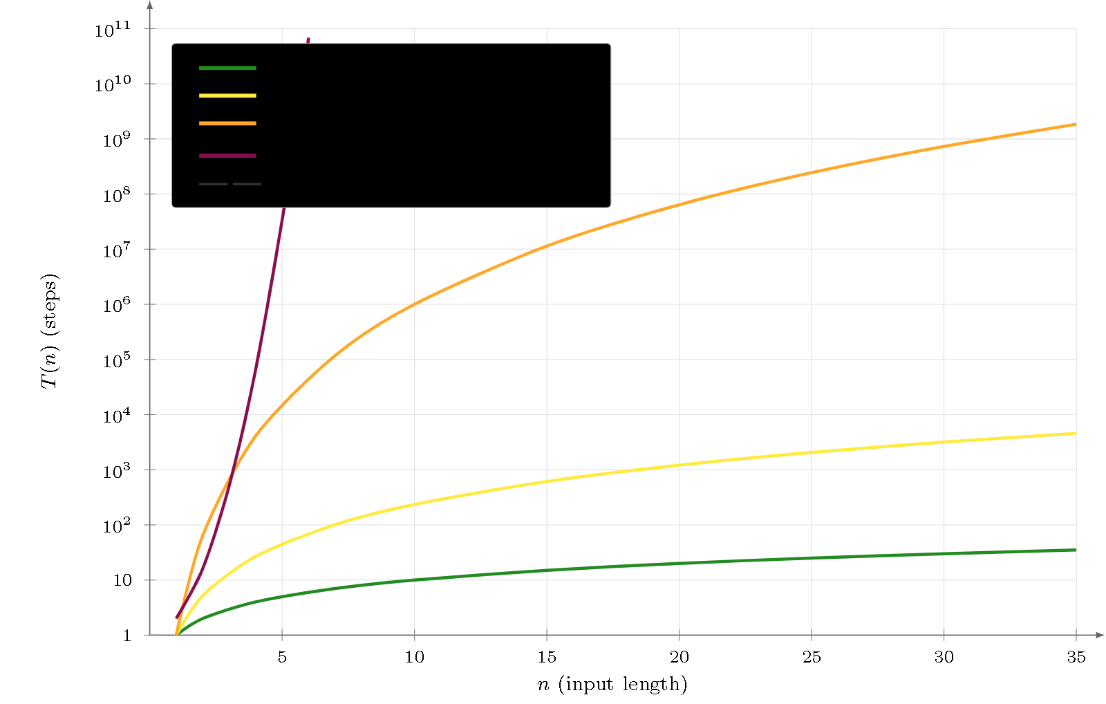
Figure 3 — Membership decision, semi-logarithmic scale. Polynomial bounds ($k=3$ slope 1, $k=2$ slope 2.37, $k=2^+$ slope 6) are straight lines; the exponential bound for CSG ($k=1$) diverges from $n\approx6$. Undecidability ($k=0$) cannot be represented on the axis.
Construction of one tree
Once membership is decided, producing one witness tree costs only a constant factor more than the decision, at all levels: decision algorithms maintain a pointer table (the chart) which simply needs to be traversed backwards to reconstruct the tree in an additional $O(n)$. Subtlety: if the string is ambiguous (multiple valid trees), producing one tree requires an arbitrary choice — but the asymptotic cost does not change.
Enumeration of all trees
Here, the problem changes nature: everything must be listed, so the cost is bounded by the output.
- Regular: only one tree per string → $O(n)$.
- CFG: the number of trees for an ambiguous string follows Catalan numbers, $C_n \sim 4^n/n^{3/2}\sqrt\pi$ — exponential. (A sentence with $k$ prepositional phrases admits $C_k$ attachments: $C_3=5$, $C_4=14$, $C_{10}=16\,796$.) Billot & Lang (1989) compact the set into a shared forest in $O(n^3)$ space, but explicitly extracting the trees remains $O(4^n)$.
- TAG/MCFG: analogous, $O(4^n)$ or worse; shared forest in $O(n^6)$.
- CSG: $O(2^{n^2})$, like the decision.
- RE: undecidable, and the number of trees can be infinite.
Table 2 — Enumeration of all trees.
Class Explicit enumeration Compact representation $k=3$ $O(n)$ $O(n)$ (single tree) $k=2$ $O(4^n)$ (Catalan) $O(n^3)$ shared forest (Billot & Lang) $k=2^+$ $O(4^n)$ or worse $O(n^6)$ shared forest $k=1$ $O(2^{n^2})$ — (same bound) $k=0$ undecidable / infinite —
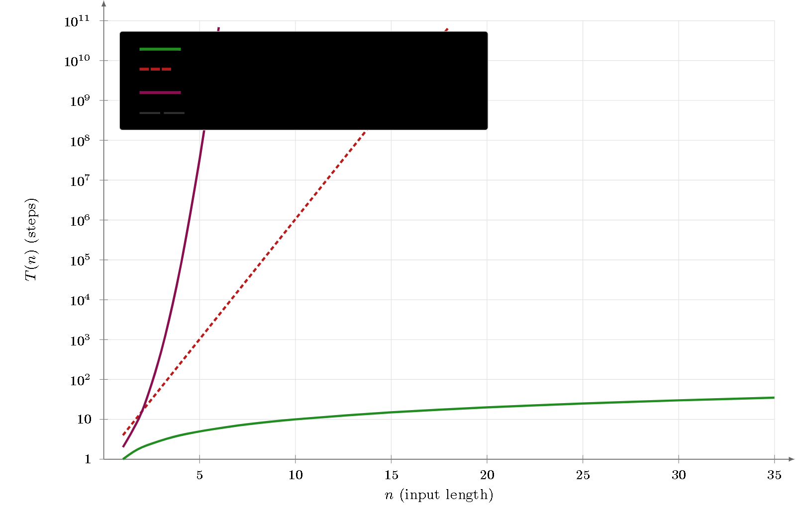
Figure 4 — Explicit enumeration of all trees. To be compared with Figure 3: for $k=3$ the curve is identical (one tree per string), but from $k=2$ the $O(4^n)$ bound (Catalan) diverges much faster than the $O(n^{2,37})$ of the decision. This is the “second dimension of difficulty”: the combinatorial explosion of the number of trees to produce.
3. Generation side
Free generation
Applying rules without a target, counting derivation steps: this is $\mathcal{O}(n)$ for all monotonic classes ($k=3$ to $k=1$) — even a Turing grammar derives freely in linear time. Free generation is immune to climbing the hierarchy. (For non-monotonic $k=0$, derivation may not terminate.)
Terminating example generation
Producing a complete string of the language. The cost remains polynomial wherever derivation terminates:
- Regular: $\Theta(n)$.
- CFG: $O(n)$ to $O(n^2)$.
- TAG/MCFG: $O(n^2)$ to $O(n^3)$.
- CSG: $O(n^3)$ — polynomial, whereas CSG decision is PSPACE-complete. This is the first strong manifestation of asymmetry in favor of generation.
Table 3 — Terminating Example Generation.
Class Total cost Characterization $k=3$ $\Theta(n)$ identical to decision $k=2$ $O(n)$ to $O(n^2)$ in $\mathsf{P}$ $k=2^+$ $O(n^2)$ to $O(n^3)$ in $\mathsf{P}$ $k=1$ $O(n^3)$ in $\mathsf{P}$ — strong contrast with PSPACE-complete decision $k=0$ unbounded semi-decidable

Figure 5 — Terminating example generation. Everything remains polynomial (slopes 1, 2, 3) for monotonic classes. To be compared with Figure 3: generation is strictly faster than decision for $k=2^+$ and $k=1$, and the gap becomes qualitative at $k=1$ (polynomial vs PSPACE-complete).
Generation under semantic constraint
Here, the produced string must additionally satisfy an external constraint (a target meaning, a format). And the profile changes radically:
- Regular: remains polynomial (intersection of automata, Mohri 1997).
- Pure CFG: polynomial if semantics are compositional. But with feature structures / unification (the standard case for linguistic grammars: LFG, HPSG), Kay (1996) shows it is exponential: a word with $k$ modifiers generates $2^k$ candidates. Brew (1992) formally proves NP-completeness (reduction from 3-Dimensional Matching) on a minimal schema.
- TAG/MCFG: inherits the exponential argument.
- CSG: NP-hard to PSPACE-hard (Barton et al. 1987).
- RE: undecidable.
Table 4 — Generation under Semantic Constraint.
Class Bound Source $k=3$ Regular polynomial Mohri 1997 $k=2$ Pure CFG polynomial folklore $k=2$ CFG + features exponential ($2^k$) Kay 1996 $k=2$ CFG + multi-set NP-complete (proven) Brew 1992 $k=2^+$ TAG + features exponential Kay/Brew $k=1$ CSG + features NP-hard to PSPACE-hard Barton 1987 $k=0$ RE undecidable Turing 1936

Figure 6 — Generation under semantic constraint. Polynomial for regular and pure CFGs, but the addition of features shifts complexity to exponential from $k=2$ (NP-complete, Brew 1992). To be compared with Figure 3: here generation exceeds decision from $k=2$ — the visual manifestation of the sign reversal.
4. The sign reversal
Let’s put the three generation sub-problems side by side with recognition:
- Free generation and terminating example generation: polynomial up to and including $k=1$. Here, “generating is easy” is true.
- Generation under semantic constraint: NP-complete from $k=2$ (with features), whereas membership decision remains polynomial up to $k=2^+$.
In other words: for constrained generation, the asymmetry reverses — generating becomes harder than parsing. This is not a figment of the imagination: Brew (1992) formally proves it. The slogan “generation is easy, parsing is hard” is therefore generally false: the asymmetry changes nature depending on the sub-problem, not just the class. (This reversal is materialized today in LLMs constrained by format or factuality — see L18.)
5. Synthesis: differential coupling
We can now compare the two sides. Table 5 confronts the two most contrasting focal cases:
Table 5 — Membership Decision vs. Terminating Example Generation.
Class Membership Decision Example Generation Gap $k=3$ $\Theta(n)$ $O(n)$ none $k=2$ $O(n^3)$ → $O(n^{2{,}37})$ $O(n)$ to $O(n^2)$ polynomial $k=2^+$ $O(n^6)$ $O(n^2)$ to $O(n^3)$ polynomial ($n^3$ to $n^4$) $k=1$ PSPACE-complete $O(n^3)$ $\mathsf{P}$ vs $\mathsf{PSPACE}$ separation $k=0$ undecidable unbounded decidability separation
And the two heatmaps (Figure 7) deploy the six complete sub-problems. This is where differential coupling becomes obvious: the generation matrix varies mainly along the rows (sensitive to the sub-problem), while the recognition matrix varies mainly along the columns (sensitive to the class).


Figure 7 — The two heatmaps: generation (top) and recognition (bottom). Rows = the three sub-problems on each side; columns = the five Chomsky classes. Generation (top) varies mainly along the rows (free → terminating → constrained): it is sensitive to the sub-problem. Recognition (bottom) varies mainly along the columns: it is sensitive to the class — except for the “all trees” row, which also explodes with the class (Catalan). This is differential coupling.
What this means concretely:
- Increasing the expressive power of the grammar penalizes parsing, but leaves free generation intact.
- Increasing constraints on the output penalizes generation, but not parsing (which is always constrained by its input).
This is the formalization of the intuition from L13: the parser is always constrained (the input is given, non-negotiable), while the generator may or may not constrain itself.
6. Musical example continued + an honest counter-argument
Continued example. For a musical grammar of level $k=2^+$ (typical of polyphonic structure grammars), recognizing a score of length $n$ costs at worst $O(n^6)$, whereas generating an arbitrary excerpt requires $O(n^2)$ to $O(n^3)$. For 100 measures ($n\approx100$), the difference is $10^6$ to $10^8$ — significant but manageable. If arbitrary global constraints were added (transition to $k=1$), recognition would become PSPACE-complete: no polynomial algorithm would exist to decide if an excerpt belongs to the language.
Counter-argument. “But for CFGs, the gap is only $n^{0,37}$ if we consider Valiant, and it disappears for LL/LR subclasses which parse in $O(n)$.” This is accurate — and instructive.
Resolution. This illustrates why intrinsic bounds and best known algorithms must be distinguished. The $O(n^\omega)$ bound for CFGs is conditional on the conjecture about $\omega$; if $\omega=2$ were proven, CFG asymmetry would collapse. For LL/LR subclasses, the gap indeed disappears — which confirms that D1 depends on the precise class, not just the level $k$. But the $\mathsf{P}$ vs $\mathsf{PSPACE}$ separation (CSG) and decidable vs undecidable (RE) do not depend on any algorithmic hypothesis: they are intrinsic.
7. In music
Differential coupling is directly observed in musical systems:
- BP3 in PROD mode (I2): free generation — fast regardless of the expressive power of the rules (first row of the generation heatmap, all green).
- BP3 in ANAL mode: the same grammar parses — complexity now depends on the class of rules (recognition heatmap, sensitive to columns).
- GTTM (M6): pure analytical parsing with context-sensitive rules → right columns of the recognition matrix.
- Constrained neural generation (format, factuality): modern illustration of the sign reversal — generating under constraint becomes costly again.
The matrix explains why musical systems are predominantly unidirectional (L16): for the same grammar, the two directions have radically different performance profiles.
Key takeaways
- “Generation” and “recognition” hide six distinct sub-problems with very different costs — they must be separated before any numbers.
- Always distinguish intrinsic bound (the problem’s difficulty) and best known algorithm (which can be improved). CFG parsing is $O(n^3)$ with CYK, but intrinsically $O(n^\omega)$.
- Recognition: decision and one-tree follow the class ($\Theta(n)$ → $O(n^\omega)$ → $O(n^6)$ → PSPACE-c → undec.); all trees explodes in $O(4^n)$ (Catalan).
- Generation: free and terminating remain polynomial wherever derivation terminates — including at $k=1$, where decision is nevertheless PSPACE-complete.
- Sign reversal: generation under semantic constraint becomes NP-complete from $k=2$ (Brew 1992) — harder than recognition. The slogan “generation is easy” is false.
- Differential coupling: recognition ← sensitive to the class; generation ← sensitive to the sub-problem. This is the true mechanism of asymmetry.
Further reading
Computational Complexity
- Younger, D.H. (1967). “Recognition and Parsing of Context-Free Languages in Time $n^3$.” Information and Control, 10(2), 189–208 — CYK.
- Valiant, L.G. (1975). “General Context-Free Recognition in Less than Cubic Time.” JCSS, 10(2), 308–315 — reduction to matrix multiplication.
- Williams, V.V. et al. (2024). “New Bounds for Matrix Multiplication.” — $\omega \le 2{,}371552$.
- Satta, G. (1994). “Tree-Adjoining Grammar Parsing and Boolean Matrix Multiplication.” Computational Linguistics — $O(n^6)$ for TAG.
- Savitch, W.J. (1970). “Relationships Between Nondeterministic and Deterministic Tape Complexities.” JCSS — CSL ⊆ DSPACE($n^2$).
- Kuroda, S.-Y. (1964). “Classes of Languages and Linear-Bounded Automata.” Information and Control — CSL = NLBA.
- Hopcroft, J.E., Motwani, R. & Ullman, J.D. (2006). Introduction to Automata Theory. Addison-Wesley.
Constrained Generation
- Kay, M. (1996). “Chart Generation.” ACL — exponential generation with features.
- Brew, C. (1992). “Letting the Cat Out of the Bag: Generation for Shake-and-Bake MT.” COLING — proven NP-completeness.
- Barton, G.E., Berwick, R.C. & Ristad, E.S. (1987). Computational Complexity and Natural Language. MIT Press.
- Mohri, M. (1997). “Finite-State Transducers in Language and Speech Processing.” Computational Linguistics — linear output of transducers.
Ambiguity
- Billot, S. & Lang, B. (1989). “The Structure of Shared Forests in Ambiguous Parsing.” ACL — shared forests in $O(n^3)$.
In the corpus
- L1 — The levels and their automata
- L9 — Type 2+: TAG, CCG, MCFG
- L13 — Overview of asymmetry (6 dimensions)
- L15 — Mathematical formalizations
- L16 — Why bidirectionality was not transferred
- L18 — The sign reversal: when generation surpasses parsing
- M6 — GTTM: the analytical paradigm applied
Glossary
- Intrinsic bound: characterization of the problem’s difficulty itself ($\Theta(f)$ or complexity class), which no algorithm can beat unless a conjecture is overturned.
- Bound of the best known algorithm: ceiling reached by the best algorithm published to date; can be improved.
- Differential coupling: generation and recognition are sensitive to both axes (class × sub-problem), but with an inverted primary sensitivity.
- Membership decision: determining whether a string belongs to the language (yes/no) — the reference bound on the recognition side.
- Generation under semantic constraint: producing a string that additionally satisfies an external constraint. NP-complete from $k=2$ with features (Brew 1992).
- Catalan numbers: $C_n \sim 4^n/n^{3/2}\sqrt\pi$ — count the derivation trees of an ambiguous CFG string.
- PSPACE-complete: solvable in polynomial space, but with no known or likely polynomial-time algorithm. CSG membership decision is PSPACE-complete.
- Sign reversal: for constrained generation, the asymmetry reverses — generating becomes harder than parsing.
- $\omega$: exponent of matrix multiplication, $\le 2{,}371552$ (Williams et al. 2024). Bounds CFG parsing via Valiant.
Prerequisites: L1, L13, L15
Reading time: 18 min
Tags: #complexity #asymmetry #heatmap #differential-coupling #Chomsky #matrix #sign-reversal