L17) The Complexity Matrix
Two Orthogonal Axes to Understand Asymmetry
In L15, we saw that generation is $\mathcal{O}(n)$ and parsing is $\mathcal{O}(n^3)$ for context-free grammars. But this formulation is misleading: it reduces each operation to a single number. In reality, complexity depends on two independent axes — the grammar class and the task specification. When these two axes are crossed in a matrix, a pattern emerges that reveals the true mechanism of asymmetry.
Where does this article fit in?
This article is a deeper dive into the first dimension (D1, Complexity) of the generation-recognition asymmetry (L13, L15). Where L15 presented a simple table — $T_{\text{gen}}$ linear versus $T_{\text{parse}}$ which explodes — this article deploys complexity across two axes and shows why asymmetry is not a simple speed difference but a differential coupling between the two operations and their parameters.
Why is this important?
Saying “generation is easy, analysis is hard” is a slogan, not an explanation. It’s even false in some cases: constrained generation can be as difficult as parsing (NP-hard). And parsing of regular languages is as fast as generation (linear).
What is true is that the two operations are not sensitive to the same parameters. Generation reacts to the degree of constraint imposed on it. Recognition reacts to the expressive power of the grammar. This difference in sensitivity — the differential coupling — is the true mechanism of asymmetry.
The idea in one sentence
The complexity of each operation is a product of two orthogonal axes — grammar class (Chomsky) × task specification — but generation is primarily sensitive to the task axis while recognition is primarily sensitive to the grammar axis.
Let’s explain step by step
1. The two axes
Each operation — generation or recognition — operates on a grammar of a certain class ($k$, the level in the Chomsky hierarchy: Type 3, Type 2, Type 2+, Type 1, Type 0 — cf. L1) and with a certain task specification — what it is asked to do.
For generation, the task specification ranges from the freest to the most constrained:
| Task Level | What is requested |
|---|---|
| Free | Apply rules without an objective — explore the language |
| Terminating | Produce a complete string (without non-terminals) |
| Constrained | Produce a specific string $w \in L(G)$ |
For recognition, the task specification ranges from the simplest question to the most complete:
| Task Level | What is requested |
|---|---|
| Membership | Is the string in the language? (yes/no) |
| One tree | Find a derivation structure |
| All trees | Enumerate all possible structures |
2. The generation matrix
When we cross the 3 task levels with the 5 grammar classes, we get a 3×5 matrix. Each cell contains the time complexity. Let’s color it like a heatmap — from green ($\mathcal{O}(n)$, fast) to dark gray (undecidable):
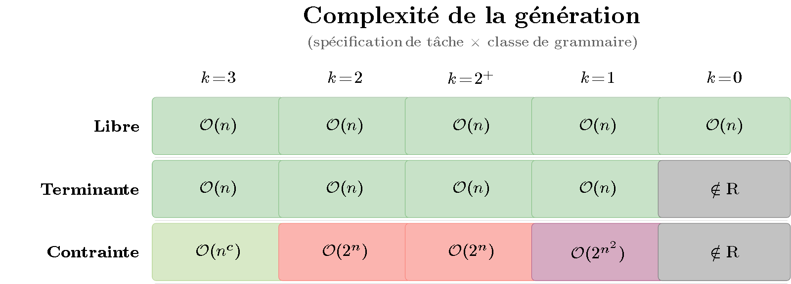
Figure 1 — Heatmap of generation complexity. Rows represent task specification (free, terminating, constrained); columns represent grammar class (Type 3 to Type 0). Color ranges from green ($\mathcal{O}(n)$, fast) to dark gray (undecidable). Key observation: the color varies mainly along the rows — it is the degree of constraint, not the grammar class, that determines the difficulty.
What the matrix shows:
- Row 1 (Free): everything is green. Free generation is linear regardless of the grammar’s power — even a Turing grammar can derive freely in $\mathcal{O}(n)$.
- Row 2 (Terminating): almost all green, except Type 0 (gray) — for recursively enumerable grammars, it is undecidable whether a derivation will reach a terminal word.
- Row 3 (Constrained): this is where the colors heat up. Producing a specific string is NP-hard from Type 2 ($\mathcal{O}(2^n)$) and worsens with expressive power.
The color gradient is horizontal: difficulty varies from one row to another, not from one column to another. Generation is sensitive to the task.
3. The recognition matrix
Same exercise for recognition:
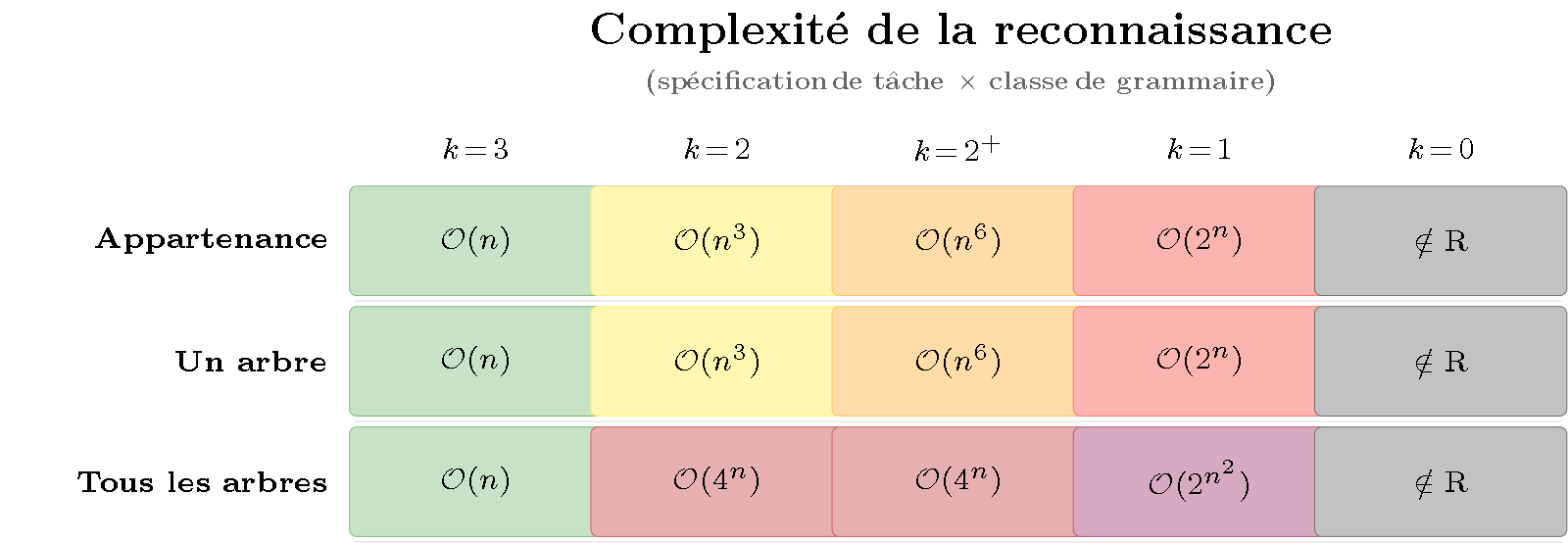
Figure 2 — Heatmap of recognition complexity. Same structure as Figure 1 but for parsing. Key observation: the color varies mainly along the columns — it is the grammar class (Chomsky hierarchy), not the task specification, that determines the difficulty.
What the matrix shows:
- Column 1 ($k=3$, regular): everything is green. Regular languages are parsed as quickly as they are generated — no asymmetry.
- Column 2 ($k=2$, context-free): yellow for membership and one tree ($\mathcal{O}(n^3)$), dark red for all trees ($\mathcal{O}(4^n)$ — Catalan numbers, cf. L15 §3).
- Columns 3-5: red and gray dominate. The more expressive the grammar, the more costly parsing is — regardless of the task specification.
The color gradient is vertical: difficulty varies from one column to another, not from one row to another (except the third row which adds the combinatorial explosion of multiple trees). Recognition is sensitive to the grammar.
4. Differential coupling
Comparing the two matrices reveals the fundamental mechanism:
| Primary sensitivity axis | Secondary axis |
|---|---|
| Generation | Task specification (rows) |
| Recognition | Grammar class (columns) |
This is what we call differential coupling: both operations are affected by both axes, but with an inverted primary sensitivity. Free generation remains $\mathcal{O}(n)$ even for a Turing grammar — it is immune to increased expressiveness. Parsing, however, is immediately affected by each jump in the Chomsky hierarchy.
In other words:
- Increasing the expressive power of the grammar makes parsing more difficult but leaves free generation intact.
- Increasing the constraints on the output makes generation more difficult but does not affect parsing (which is always constrained by the input).
This is the formalization of the intuition from L13: the parser is always constrained (the input is given, non-negotiable), while the generator may or may not constrain itself.
5. The divergence curve
The two matrices can be summarized in a single curve when we fix the most common task (membership for parsing, free generation for production) and vary the grammar class:
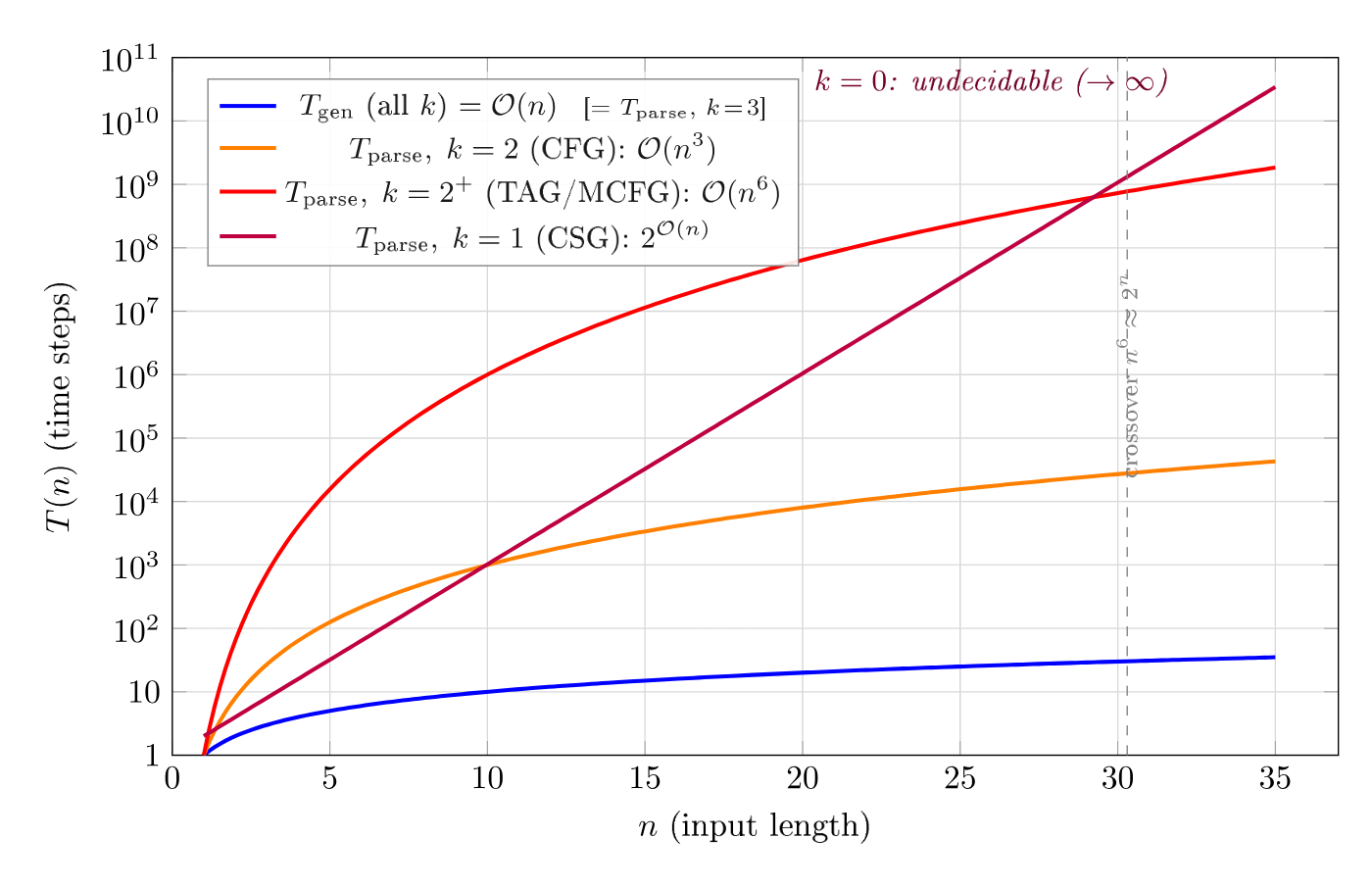
Figure 3 — The complexity gap (semi-log scale). Seven curves corresponding to the complexity levels identified in the heatmaps, with the same color palette. Polynomial bounds appear as straight lines; exponential bounds diverge upwards. The dashed vertical line marks undecidability ($\notin \mathrm{R}$).
On a semi-logarithmic graph (vertical axis in $\log_{10}$), polynomial complexities ($n$, $n^3$, $n^6$) are straight lines whose slope increases with the exponent. Exponential complexities ($2^n$, $4^n$, $2^{n^2}$) diverge upwards. For an input of 20 symbols:
| Complexity | Operations |
|---|---|
| $\mathcal{O}(n)$ | 20 |
| $\mathcal{O}(n^3)$ | 8,000 |
| $\mathcal{O}(n^6)$ | 64,000,000 |
| $\mathcal{O}(2^n)$ | 1,048,576 |
| $\mathcal{O}(4^n)$ | $\approx 10^{12}$ |
Asymmetry is not a constant factor: it grows with expressive power. This is why mildly context-sensitive formalisms ($k = 2^+$, cf. L9) — those that dominate computational linguistics — are in a critical zone: expressive enough to capture interesting linguistic phenomena, but with parsing in $\mathcal{O}(n^6)$ which makes large-scale applications difficult.
6. In music
Differential coupling is directly observed in musical systems:
- BP3 in PROD mode (I2): the grammar freely generates bol sequences. Regardless of the expressive power of the rules, generation remains fast — we are in the first row of the matrix (all green).
- BP3 in ANAL mode: the same grammar analyzes a given sequence. Complexity now depends on the expressive power of the rules — we are in the right matrix, where columns determine the color.
- GTTM (M6): pure analytical parsing. Preference rules are context-sensitive (decisions depend on global context), which places GTTM in the right columns of the recognition matrix — where red dominates.
- Neural generators (Jukebox, MusicGen): free generation in $\mathcal{O}(n)$ per token, but with a colossal training cost that implicitly encodes all analytical work.
The matrix explains why musical systems are predominantly unidirectional (L16): differential coupling means that the two directions have radically different performance profiles for the same grammar.
Key takeaways
- The complexity of each operation depends on two orthogonal axes: the grammar class (Chomsky hierarchy) and the task specification.
- The generation matrix shows a horizontal gradient (sensitive to the task); the recognition matrix shows a vertical gradient (sensitive to the grammar).
- This differential coupling is the true mechanism of asymmetry: increasing expressive power penalizes parsing but not free generation; increasing constraints penalizes generation but not parsing.
- Asymmetry grows with expressive power: from none (Type 3) to infinite (Type 0).
- In music, differential coupling explains why the same BP3 grammar generates quickly (PROD) but analyzes more slowly (ANAL).
To go further
Computational complexity
- Aho, A.V., Sethi, R. & Ullman, J.D. (1986). Compilers: Principles, Techniques, and Tools. Addison-Wesley — CYK, Earley, LL, LR complexities.
- Hopcroft, J.E. & Ullman, J.D. (1979). Introduction to Automata Theory, Languages, and Computation. Addison-Wesley — fundamental results.
- Satta, G. (1994). “Tree-Adjoining Grammar Parsing and Boolean Matrix Multiplication.” Computational Linguistics — $\mathcal{O}(n^6)$ complexity for TAG.
Constrained generation
- Barton, G.E., Berwick, R.C. & Ristad, E.S. (1987). Computational Complexity and Natural Language. MIT Press — NP-completeness proofs.
- Song, L. et al. (2016). “AMR-to-text Generation as a Travelling Salesman Problem.” EMNLP — NP-hard generation.
- Adolfi, F., Wareham, T. & van Rooij, I. (2022). “Intractability in Parsing and Segmentation.” — intrinsic NP-hardness.
In the corpus
- L1 — The hierarchy levels and their automata
- L9 — Type 2+: TAG, CCG, MCFG
- L13 — Overview of asymmetry (6 dimensions)
- L15 — Mathematical formalizations of the 6 dimensions
- L16 — Why bidirectionality has not been transferred
- M6 — GTTM: the analytical paradigm applied
Glossary
- Grammar class ($k$): The level in the Chomsky hierarchy. $k = 3$ (regular), $k = 2$ (context-free), $k = 2^+$ (mildly context-sensitive), $k = 1$ (context-sensitive), $k = 0$ (recursively enumerable).
- Differential coupling: The fact that generation and recognition are both sensitive to both axes (grammar class and task specification), but with an inverted primary sensitivity. Generation reacts primarily to the task; recognition reacts primarily to the grammar.
- Constrained generation: Generation that must produce a specific string $w$, not just any string from the language. Can be NP-hard from Type 2.
- Free generation: Generation without an output objective — rules are applied, and the result is observed. Always $\mathcal{O}(n)$, regardless of grammar class.
- Heatmap: Visual representation of a matrix where color codes the intensity of a value. Here, green codes low complexity ($\mathcal{O}(n)$) and dark gray codes undecidability.
- Task specification: What the operation is asked to produce. For generation: free, terminating, constrained. For recognition: membership, one tree, all trees.
Prerequisites: L1, L13, L15
Reading time: 12 min
Tags: #complexity #asymmetry #heatmap #differential-coupling #Chomsky #matrix
← Back to index