M6) Hierarchical Structure in Music
GTTM Demystified
When you listen to a symphony, how do you know that a passage is a “conclusion”? How do you perceive that a theme “returns”? GTTM attempts to formalize these intuitions that we all have.
Where does this article fit in?
This article elaborates on the ideas from M4 by detailing GTTM — the most advanced theory for formalizing musical perception. It also serves as a theoretical foundation for bp2sc, the transpiler (source-to-source code translator) connecting I2 (Bol Processor, version 3) to I3 (see B7).
What is GTTM?
GTTM stands for Generative Theory of Tonal Music. It is a theory developed by Fred Lerdahl and Ray Jackendoff in 1983 that attempts to formally describe how a listener perceives and mentally organizes Western tonal music. The term “generative” refers to Chomsky’s generative linguistics: just as a grammar can “generate” all possible sentences of a language, GTTM proposes a set of rules that can “generate” all valid perceptual structures of a musical piece.
Why is it important?
Imagine you had to program software capable of automatically analyzing a musical piece: identifying phrases, themes, moments of tension and resolution. Where would you start?
In 1983, Fred Lerdahl (composer) and Ray Jackendoff (linguist) published A Generative Theory of Tonal Music (GTTM), an ambitious attempt to formalize how we perceive musical structure. Their theory profoundly influenced computational musicology, automatic musical analysis, and even computer-assisted composition.
Understanding GTTM means understanding why music seems to have “meaning” to us, even without words.
The idea in one sentence
GTTM models our perception of tonal music through four parallel hierarchical structures: grouping, meter, time-span reduction, and prolongational reduction.
Let’s explain step by step
Example 1: Reading a sentence
Before tackling music, let’s consider reading. When you read:
“Le petit chat gris dort sur le canapé rouge.” (The small grey cat sleeps on the red sofa.)
Your brain doesn’t process this sentence word by word. It automatically constructs a structure:
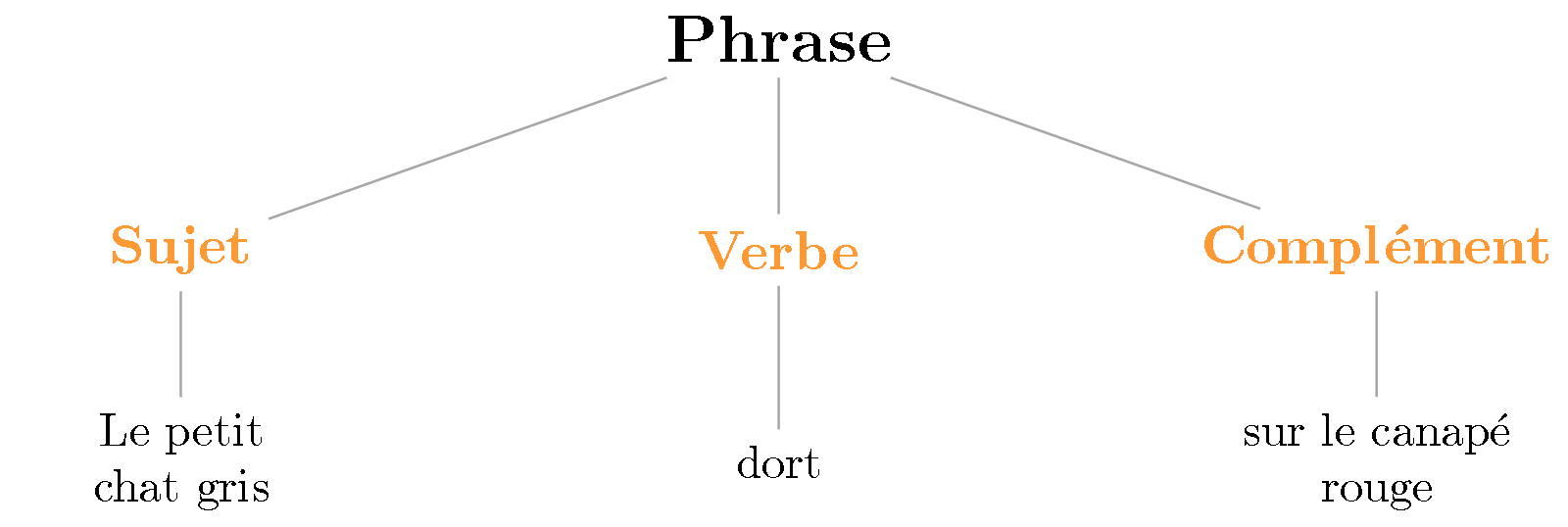
Figure 1 — Syntactic tree of a French sentence. Our brain automatically constructs this hierarchy: “petit” modifies “chat”, not “dort”.
You know that “petit” (small) modifies “chat” (cat), not “dort” (sleeps). You know that “rouge” (red) describes the “canapé” (sofa), not the “chat” (cat). This hierarchical structure is implicit — you don’t consciously calculate it.
Example 2: Hearing a melody
The same thing happens in music. Take “Au clair de la lune” (By the light of the moon):
Au clair de la lu-ne, mon a-mi Pier-rot
|__________________|  |_______________|
    Phrase A              Phrase B

Prê-te-moi ta plu-me pour é-crire un mot
|__________________|  |_______________|
    Phrase C              Phrase D
You naturally perceive these four phrases, even if no one told you. And you perceive that A+B form a larger unit (the “question”) which contrasts with C+D (the “answer”).
It is this hierarchical structure that GTTM attempts to formalize.
The four components of GTTM
1. Grouping Structure
Fundamental question: How do notes group together into motives, phrases, sections?
The grouping structure is the most intuitive component of GTTM. It answers a simple question: when you listen to music, how do you know where a “phrase” begins and where it ends?
Think of punctuation in a text. Without commas or periods, a long string of words would be difficult to understand. In music, there is no visible punctuation, but our brain naturally “hears” separations. The grouping structure models these perceived boundaries.
It organizes music into nested units, like Russian dolls:
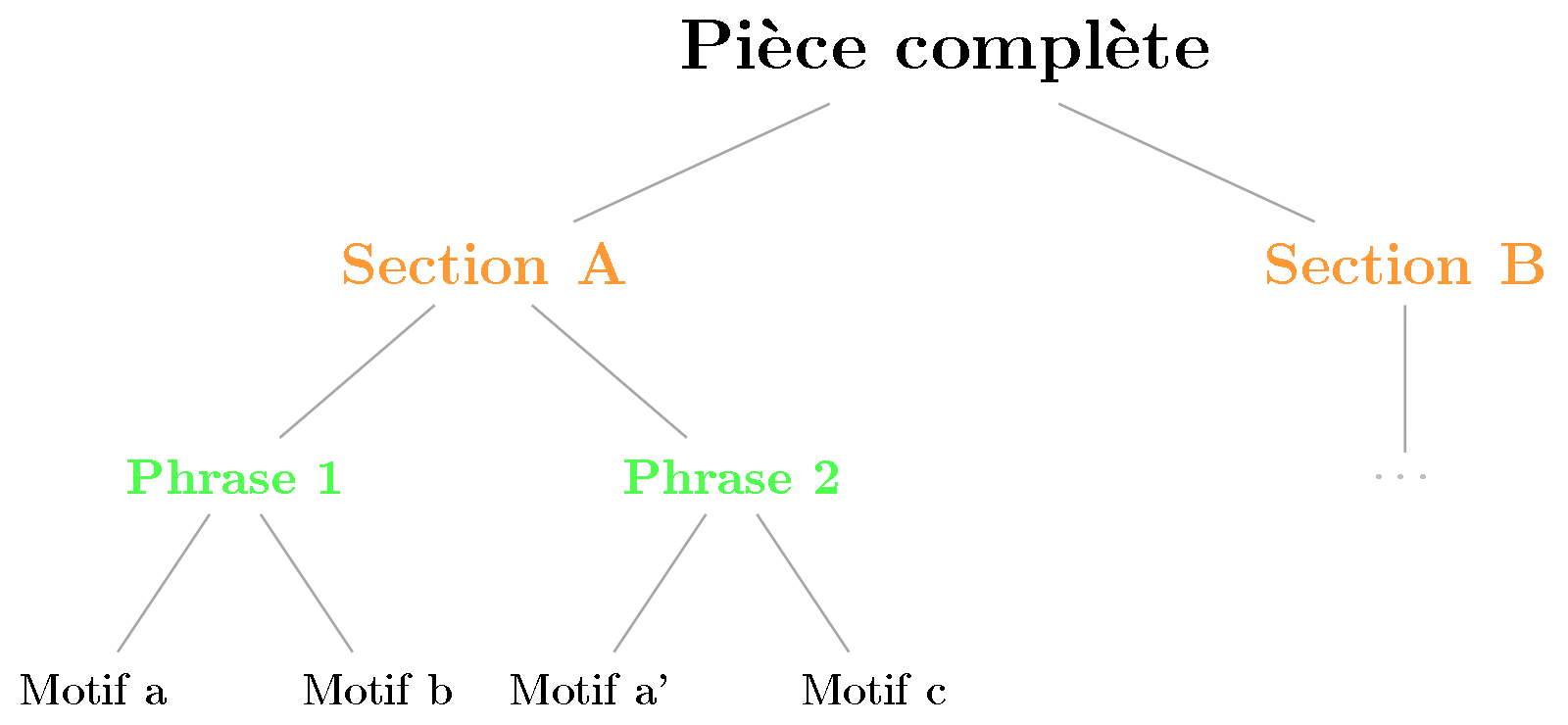
Figure 2 — GTTM grouping structure: music is organized into nested units like Russian dolls, from the entire piece down to individual motives.
Grouping Preference Rules (GPR):
GTTM proposes rules that describe our perceptual tendencies. These rules are not absolute laws but preferences: they indicate what we tend to perceive, not what we necessarily perceive.
Why “preference rules”?
Unlike strict grammar rules (“a sentence must have a verb”), preference rules are statistical tendencies. They can contradict each other! For example, GPR 2a might suggest a boundary in one place, while GPR 3a suggests another. In this case, GTTM proposes that the rules “combine” and the perceived boundary is the one with the most converging cues. This is exactly like in visual perception: multiple cues can add up or contradict each other.
The main GPRs:
- GPR 2a (Proximity): A silence or lengthening between two notes suggests a group boundary. Example: in “Frère Jacques”, the pause after “dor-mez-vous” creates a clear separation.
- GPR 2b (Change of Attack): An abrupt change in the mode of attack (from legato to detached) suggests a boundary.
- GPR 3a (Register): A large melodic interval (typically more than 7 semitones, i.e., a fifth, the interval between C and G) suggests a boundary. Example: if a melody goes C-D-E then jumps to high C, this jump creates a perceptual break.
- GPR 3c (Dynamics): A sudden change in volume (piano, soft, to forte, loud, or vice-versa) suggests a boundary. Example: the entrance of the tutti (full orchestra) after a solo passage.
- GPR 3d (Articulation): A change in articulation (legato, i.e., connected playing, to staccato, i.e., detached notes) suggests a boundary. Example: a sung phrase followed by staccato notes.
Example with “Au clair de la lune”:
Au clair de la lu- | ne      (pause = GPR 2a)
Mi mi mi ré mi    | do      (long note + change of direction)
The silence after “lu-” and the long note on “ne” create a group boundary.
2. Metrical Structure
Fundamental question: Which beats are “strong” and which are “weak”?
The metrical structure models our perception of the music’s “beat”. Be careful: this is not the time signature written on the score (4/4, 3/4…), but the hierarchy of accents that we mentally perceive.
Imagine tapping your foot while listening to music. You don’t tap on every note, but on certain regular points. And among these points, some seem more “important” than others (the “one” of each measure, for example). It is this hierarchy that the metrical structure captures.
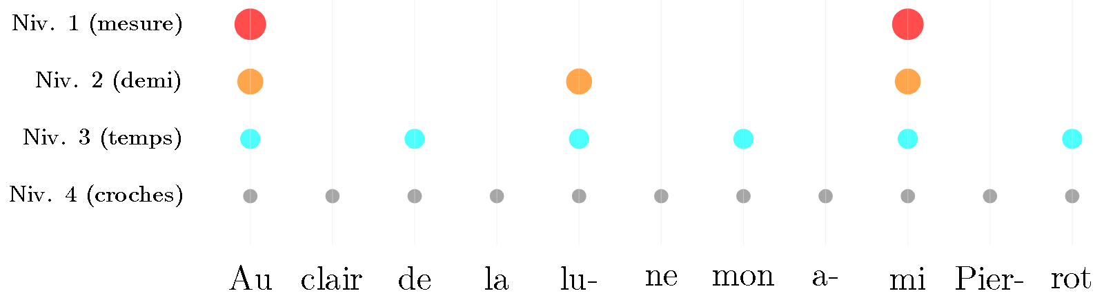
Figure 3 — Multi-level metrical grid for “Au clair de la lune”. A “strong” beat appears at multiple levels of the hierarchy.
A “strong” beat is a beat present at multiple levels of the hierarchy. The first beat of each measure is the strongest because it appears at all levels.
Metrical Preference Rules (MPR):
These rules describe how we infer the metrical structure from musical events:
- MPR 1 (Coincidence): Musical events (note attacks) must coincide with beats of the metrical grid. If you hear a note, your brain assumes it falls on a beat.
- MPR 5 (Length): Long notes tend to fall on strong beats. Example: in “Happy Birthday”, the “birth-” of “birthday” is long AND on a strong beat.
- MPR 6 (Harmony): Important chord changes (especially cadences, harmonic formulas that conclude a musical phrase) prefer strong beats. Example: the final chord of a perfect cadence (dominant-tonic progression, V-I) almost always falls on a strong beat.
3. Time-Span Reduction
Fundamental question: Among the notes in a group, which one is the most “important”?
Time-span reduction answers a classic musicological question: if you had to “summarize” a melody, which notes would you keep?
This component builds a reductional tree: each group has a “head” (structurally important note), and the other notes are elaborations of this head. An elaboration is a note that “decorates” or “ornaments” the head without changing its structural meaning.
What is a reductional tree?
A reductional tree is a hierarchical structure where:
- At the lowest level, you have all the notes of the piece
- At each higher level, the less important notes are “eliminated”
- At the top, only the most structural note(s) remain (often the tonic or dominant)
It’s the musical equivalent of a text summary: you keep the essential, you eliminate the details.
Simplified example:
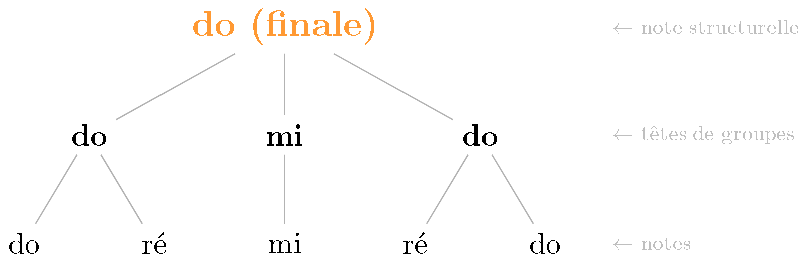
Figure 4 — Time-span reduction tree. The D’s are passing notes, E is the melodic peak, but the final C (tonic, cadential position) dominates the whole.
In this example:
- The two
Ds are passing notes (neighboring tones) — they are eliminated.Cis the head of each extreme group. Eis the melodic peak, but harmonically less stable thanC.- The final
Cprevails: it is the tonic (resting note), in a cadential position (end of phrase). It dominates the whole —Eis an elaboration (upper neighbor) ofC.
Time-Span Reduction Preference Rules (TSRPR):
- TSRPR 1 (Metrical Position): The head of a group must be on a metrically strong beat. Example: between an eighth note on the beat and an eighth note on the off-beat, the one on the beat will be preferred as the head.
- TSRPR 2 (Harmonic Stability): The head of a group must be harmonically stable (consonant, i.e., perceived as stable and “in agreement” with the harmony). Example: if a C major arpeggio contains C-E-G, the C (root) will be preferred as the head.
- TSRPR 3 (Melodic Connection): Melodically close notes (small intervals, conjunct motion, i.e., by successive whole or half steps) tend to be grouped, and the “framing” note (beginning or end of the conjunct motion) is the head. Example: in C-D-E-D-C, the E (climax) can be the head, or the C’s (framing notes) depending on the context.
4. Prolongational Reduction
Fundamental question: What are the tension and release relationships between events?
Prolongational reduction is the most abstract component of GTTM, but also the most musically significant. It captures our feeling that music “goes somewhere” and then “arrives” — what musicians call tension and resolution.
Imagine a story with a beginning, a development that builds suspense, and a final resolution. Music works similarly: some passages create expectation, others resolve it. Prolongational reduction models these relationships.
Prolongation vs. Progression
The key distinction is between prolonging (staying in the same harmonic state) and progressing (changing harmonic state):
- Prolongation: C major → a few passing notes → C major. We stay “in” C from beginning to end — the harmony doesn’t really move.
- Progression: G7 → C major. We change harmony: G7 (dominant, unstable) creates tension that resolves by arriving on C major (tonic, stable). It’s a movement, not a sustain.
Three types of connections:
- Strong prolongation: One event directly prolongs another (same harmony). Example: C major — a few melody notes — C major. The second C major is a prolongation of the first.
- Weak prolongation: One event is an “embellishment” or “neighbor” of another. Example: C major — D minor — C major. The D minor is an embellishment that decorates the C without really leaving it.
- Progression: One event creates tension towards another. Example: G7 to C major. The G7 is not a prolongation of C, it progresses towards it, creating harmonic movement.
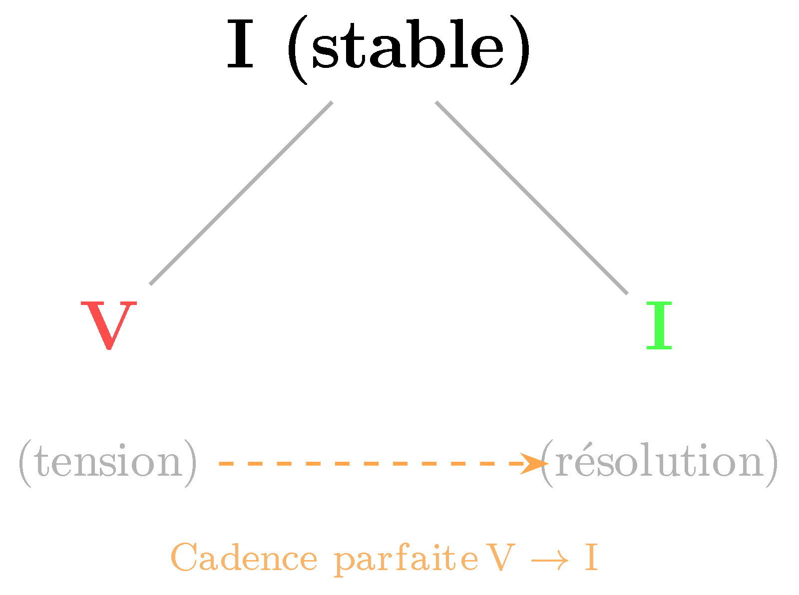
Figure 5 — Prolongational tree of a perfect cadence. The V chord (dominant) creates tension that resolves to I (tonic).
The V chord (dominant) creates tension that resolves to I (tonic). This relationship is represented in the prolongational tree.
Why trees?
The power of tree representation
What is a tree in computer science?
A tree (in computer science and mathematics) is a data structure that represents a hierarchy. Visually, it’s like an inverted family tree:
- The root is at the top (the common ancestor)
- The nodes are the intermediate elements
- The leaves are the final elements, with no descendants
- Each node (except the root) has exactly one parent
- Each node can have zero, one, or more children
In a GTTM musical tree, the root represents the entire piece, the leaves are the individual notes, and the intermediate nodes are the groups, phrases, and sections.
A tree naturally captures:
- Hierarchy: A parent node dominates its children.
- Inclusion: Children are “contained” within the parent.
- Relationships: One can trace back from any node to the root.
For music, this allows answering questions like:
- “Which phrase does this note belong to?” → Go up the grouping tree.
- “Is this passage stable or tense?” → Consult the prolongational tree.
- “What is the structural note of this section?” → Find the head in the reduction.
Comparison with a flat list
Without a tree structure, a musical piece would just be a sequence of notes:
List: C, D, E, F, G, A, B, C
With a tree:
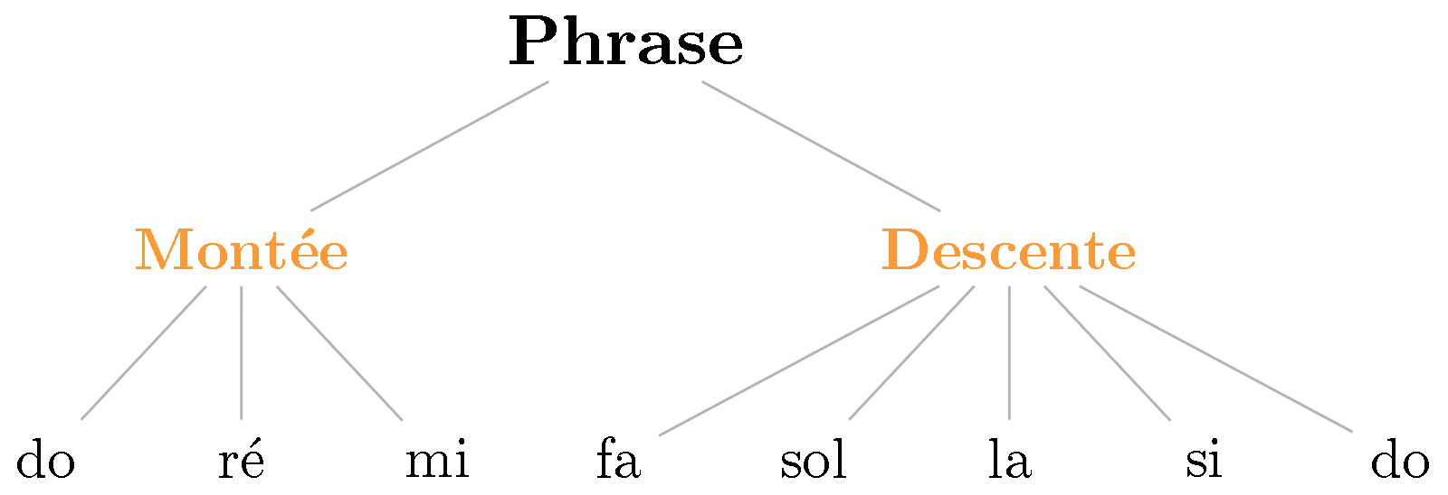
Figure 6 — Tree structure vs. flat list. The tree captures the fact that C-D-E forms a unit (ascent) which contrasts with the descent.
The tree captures the fact that C-D-E forms a unit, that this unit contrasts with the descent, etc.
Analysis vs. Generation
GTTM for analysis
GTTM was designed to analyze — to take a piece and deduce its structure. The preference rules guide this analysis:
Input: Score of "Au clair de la lune"
Process: Apply GPR, MPR, TSRPR, PRPR rules
Output: Four trees representing the perceived structure
(Note: PRPR = Prolongational Reduction Preference Rules, the preference rules for prolongational reduction.)
GTTM for generation
Can the process be reversed? Start from an abstract structure and generate a piece?
This is more difficult, because preference rules are descriptive (they describe what is perceived) and not prescriptive (they don’t say what to compose).
However, several researchers have adapted GTTM for generation:
- Hamanaka et al. created a generative system based on GTTM.
- Lerdahl himself proposed extensions in Tonal Pitch Space (2001) that are better suited for generation.
GTTM and BP3: two opposite directions
GTTM and I2 (Bol Processor) share the principle of hierarchical structure in music, but their theoretical origins and directions are independent:
- GTTM comes from cognitive linguistics (Jackendoff) applied to musical perception.
- BP3 comes from formal language theory (Chomsky, Panini) applied to musical generation.
They are complementary, not derived from each other:
| Aspect | GTTM | BP3 |
|---|---|---|
| Direction | ↑ Ascending (analysis) | ↓ Descending (generation) |
| Theoretical lineage | Cognitive linguistics (Jackendoff) | Formal languages (Chomsky, Panini) |
| Input | Musical surface (notes) | Grammar (production rules) |
| Output | Structural trees | Musical sequences |
| Rules | Preference (perceptual tendencies) | Production (deterministic or weighted) |
| Application | Western tonal music | Any music (Indian, Western…) |
In terms of abstraction levels: GTTM moves up from events to structure, BP3 moves down from grammar to events. A system that combined both would achieve a complete cycle: analyze a piece (GTTM ↑), extract a structure, then generate variations from it (BP3 ↓).
Limitations of GTTM
Focused on Western tonal music
GTTM was developed for tonal music (Bach, Mozart, Beethoven…). Its rules do not directly apply to:
- Atonal music (music without a tonal center, like Schoenberg, Webern)
- Non-Western music (Indian ragas, Indonesian gamelan)
- Electronic music (no discrete “notes”)
Formalization remains incomplete
Preference rules are often formulated qualitatively (“a large interval suggests a boundary”). But how many semitones make a “large” interval? GTTM does not always specify this.
A single idealized listener
GTTM models the perception of an “idealized competent listener”. But different listeners can perceive the same piece differently. This variability is not well captured.
Key takeaways
- GTTM proposes four parallel structures to model our musical perception:
1. Grouping (segmentation into units)
2. Meter (hierarchy of strong/weak beats)
3. Time-span reduction (important notes vs. ornaments)
4. Prolongational reduction (tension and release)
- Preference rules describe our perceptual tendencies (silences = boundaries, long notes = strong beats…).
- Tree representation naturally captures musical hierarchy and relationships.
- GTTM is designed for analysis, but its principles can be adapted for generation.
- Limitations: focused on Western tonal music, sometimes vague formalization, a single type of listener.
Further reading
- Lerdahl, F. & Jackendoff, R. (1983). A Generative Theory of Tonal Music. MIT Press. — The original work, dense but foundational.
- Temperley, D. (2001). The Cognition of Basic Musical Structures. MIT Press. — A more formal and computational reformulation of GTTM.
- Hamanaka, M., Hirata, K., & Tojo, S. (2006). “Implementing ‘A Generative Theory of Tonal Music'”. Journal of New Music Research. — On computer implementation.
- Marsden, A. (2010). “Schenkerian Analysis by Computer”. Journal of New Music Research. — On the links between GTTM and Schenkerian analysis.
Glossary
- Tree (computer science): Hierarchical data structure with a root, intermediate nodes, and leaves. Each node (except the root) has a unique parent.
- Reductional tree: Hierarchical structure where each level simplifies the lower level by keeping only the structurally important elements.
- Neighboring tone (embellishment): Ornamental note that leaves a structural note by conjunct motion and returns to it. Example: C-D-C.
- Cadence: Harmonic formula that concludes a musical phrase. The perfect cadence (V-I) is the most conclusive.
- Consonance/Dissonance: Consonance is the quality of a stable and “pleasant” sound (octave, fifth, major third). Dissonance is unstable and calls for resolution.
- Dominant (V): Fifth degree of the scale, a tension chord that calls for the tonic.
- Elaboration: A note or passage that “decorates” a structural note without changing its meaning.
- GPR (Grouping Preference Rules): Preference rules for grouping. Describe how we perceive boundaries between musical groups.
- GTTM (Generative Theory of Tonal Music): Generative theory of tonal music, developed by Lerdahl and Jackendoff (1983).
- Metric: Hierarchical organization of strong and weak beats, distinct from rhythm (note durations).
- Conjunct motion: Melodic movement by successive whole or half steps (C-D-E), as opposed to disjunct motion (leaps, like C-G).
- MPR (Metrical Preference Rules): Preference rules for metrical structure. Describe how we infer the beat grid.
- PRPR (Prolongational Reduction Preference Rules): Preference rules for prolongational reduction. Describe how we perceive tension/resolution relationships.
- Progression (harmonic): Movement from one chord to another that creates tension and a sense of direction.
- Prolongation: Relationship where a musical event extends or elaborates another without creating a new harmonic direction.
- Preference rule: A rule that indicates a perceptual tendency, not an obligation. Can conflict with other rules.
- Head: The structurally most important note of a group. The other notes in the group are elaborations of the head.
- Tonic (I): First degree of the scale, a point of rest and harmonic stability.
- TSRPR (Time-Span Reduction Preference Rules): Rules for identifying group heads in time-span reduction.
Prerequisite: M4 — Grammars and Music
Reading time: 11 min
Tags: #gttm #musical-analysis #hierarchy #lerdahl #jackendoff #cognition
Next article: B1 — PCFG: when grammars roll the dice